Implementation
Theoretical Background
Reference Documents
RD1 |
|
RD2 |
‘SKA1 Performance Assessment Report’ SKA-TEL-SKO-0001089 |
Applicable Documents
AD1 |
An improved source-subtracted and destriped 408 MHz all-sky map |
An overview of the theoretical performance of SKA Mid comprising SKA1 and MeerKAT dishes is given in RD1. A more detailed analysis is given in RD2 for an SKA Mid made up of only SKA1 dishes. We are grateful to Songlin Chen for help in navigating and understanding the documentation.
The Mid Sensitivity Calculator (SC) was originally implemented following the theoretical framework of RD1 but is moving to the more rigorous framework of RD2, though some details remain simplified.
Dish SEFD
The ‘system equivalent flux density’ (SEFD) for a single dish is the flux density of a source that produces a signal equal to the background power of the system:
where:
\(k\) is the Boltzmann constant so that \(kT_{sys}\) measures the power received from background emission and all other sources of unwanted signal within the system, that is \(T_{sys} = T_{spl} + T_{sky} + T_{rcv} + T_{cmb} + ...\)
\(\eta_A\) is the dish efficiency
\(A\) is the geometric dish area.
The 2 is there because a radio telescope measures only one polarization and it is assumed for this purpose that the other polarization has the same strength.
Array SEFD
SKA Mid is an interferometer that works by combining the signal from multiple dishes. There are 2 types of dishes involved, SKA1 and MeerKAT, with distinct characteristics. It can be shown, by adding up the signals from each baseline, that the array SEFD is given by:
where:
\(n_{\mathrm{SKA}}\) is the number of SKA antennas
\(n_{\mathrm{MeerKAT}}\) is the number of MeerKAT antennas
\(SEFD_{\mathrm{SKA}}\) is the SEFD computed for an individual SKA antenna
\(SEFD_{\mathrm{MeerKAT}}\) is the SEFD computed for an individual MeerKAT antenna.
and the assumption has been made (?) that all baselines are equally efficient.
Array Sensitivity
The ‘sensitivity’ of a radio telescope is an overloaded term. For the purpose of the SC we define the sensitivity as the minimum detectable Stokes I flux (1 \(\sigma\)). This is equal to the noise on the background power, obtained using the radiometer equation \(\sigma = SEFD / \sqrt{2 B t}\), corrected for atmospheric absorption:
where:
\(\Delta S_{min}\) is the source flux density above the atmosphere
\(\eta_s\) is the efficiency factor of the interferometer
\(B\) is bandwidth
\(t\) is integration time
\(\tau_{atm}\) is the optical depth of the atmosphere towards the target
the formula applies to the centres of fields-of-view where the dish aperture response is unity.
Dependency Tree
The devil is in the detail of calculating \(T_{sys}\) and the efficiency factors \(\eta_A\) and \(\eta_s\). Fig.1 shows how these values depend on other factors that must be estimated.
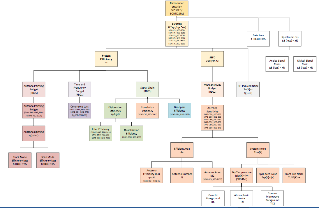
Figure 1 . The dependency tree for factors in the sensitivity calculation (from RD2).
Currently, the SC does not incorporate all the dependency factors. Those that are included are described in the following sections.
System Temperature
The system temperature is given by:
where:
and:
\(T_{spl}\) is the spillover temeprature, measuring power from the ground reaching the receiver. Currently this is set to 3K for SKA1 dishes and 4K for MeerKAT.
\(T_{rcv}\) measures noise from the receiver and electronics, depending on band and dish type.
\(T_{sky}\) is the total emission from the sky.
\(T_{CMB}\) is the cosmic microwave background, 2.73K.
\(T_{gal}\) is the Galactic astronomical emission in the target direction. \(T_{gal} = T_{408} (0.408 / \nu_{GHz})^{alpha}\) K, where \(T_{408}\) is the Galactic emission at 408MHz whose estimation is described in Brightness at 408MHz.
\(T_{atm}\) measures the brightness of the atmosphere, which depends on weather, observing frequency and elevation. \(T_{atm}\) and \(\tau_{atm}\) at the zenith are interpolated from lookup tables of results from the CASA atmosphere module, run for a grid of frequencies and weather PWVs. \(T_{atm}\) at the target elevation is estimated by relating it to the physical temperature by \(T_{phys} \sim T_{atm} (1 - \exp(-\tau_{atm}))\), where \(\tau_{atm}\) varies as \(\sec(z)\).
Brightness at 408MHz
The brightness of the astronomical background signal at 408MHz is estimated using the all-sky non source-subtracted HEALPix map described by AD1 (Fig.2). The brightness seen by a dish is calculated by multiplying map pixels that lie under the beam by the beam profile. The beam is assumed to be Gaussian, truncated at a radius equal to the FWHM.
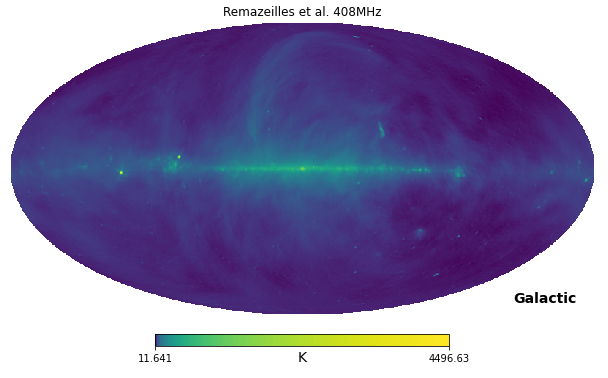
Figure 2 . The all-sky 408Mhz map from AD1, used to calculate \(T_{408}\).
Efficiencies
Aperture
Following RD2, the aperture efficiency \(\eta_A\) is given by:
where:
and:
\(\eta_{dish}\) accounts for the efficiencies attributable to the dish optics
\(\eta_{block}\) accounts for physical aperture blockage
\(\eta_{transp}\) accounts for losses by transmission through the reflector surface
\(\eta_{surface}\) accounts for all losses due to incoherent propagation through the optics, including panel roughness, systematic deformation and mis-alignment;
\(\eta_{rad.r}\) accounts for the Ohmic dielectric and scattering losses in the reflector system only
\(\eta_{feed}\) accounts for the efficiencies attributable to the feeds
\(\eta_{rad.f}\) accounts for feed mismatches and losses
\(\eta_{ill}\) is the efficiency due to the actual illumination pattern
Currently, the SC follows RD1 and calculates an overall \(\eta_{dish}\) from estimates of \(\eta_{ill}\), \(\eta_{surface}\) and \(\eta_{diffraction}\) (?).
Array
The system efficiency \(\eta_s\) is the result of multiplying together the following factors:
eta_bandpass This factor describes the loss of efficiency due to the departure of the bandpass from an ideal, rectangular shape. At present the value is set to 1.0.
eta_coherence This factor desribes the loss of efficiency due to coherence loss on a baseline.
\[\eta_{coherence} = \exp-\frac{<\phi_{\epsilon}^2 (t)>}{2} = \exp-2\pi ^2 \nu_0^2 <\tau_\epsilon ^2(t)>\]We take the coherence loss at 1s integration time, which is white phase-noise dominated. The total phase delay is due to the sum in quadrature of the phase delay of the clock and signal path on both receptors:
\[<\tau_\epsilon ^2> = <\tau_{clk,i}^2> + <\tau_{clk,j}^2> + <\tau_{dsh,i}^2> + <\tau_{dsh,j}^2>\]The signal path depends on the environment (atmosphere, gusty wind) and the calibration quality, which is quite complicated to estimate in practice. For now we adopt a value of \(\eta_{coherence} = 0.98\) at \(\nu_0 =15.4GHz\) as coherence loss for the worst case, and scale it to the frequency of observation using the given formula.
eta_correlation This factor describes the loss of efficiency due to imperfection in the correlation algorithm, e.g. truncation error. Analysis described in “SKA CSP SKA1 MID array Correlator and Central beamformer sub element Signal Processing Matlab Model” (311-000000-007) shows that the CSP correlation efficiency is almost 100% in the case of zero RFI, and better than 98% in the case of strong RFI (defined as <10% RFI in the outside visibility ?query, what does this mean).
Currently the efficiency value is set to 0.98.
eta_digitisation This factor describes the loss of efficiency due to quantization during signal digitisation. The process is independent of the telescope and environment, and depends only on the ‘effective number of bits’ (ENOB) of the system, which depends in turn on digitiser quality and clock jitter, and on band flatness.
The values used for each band are as follows:
Band
ENOB
Band Flatness (dB)
\(\eta\)
Band 1
8
6.5
0.999
Band 2
8
6.5
0.999
Band 3
6
6.5
0.998
Band 4
4
6.5
0.98
Band 5a
3
4 (in any 2.5GHz BW)
0.955
Band 5b
3
4 (in any 2.5GHz BW)
0.955
eta_point This factor describes the loss of efficiency due to dish pointing errors. Here we currently use an approximate formula:
\[\eta_{point} \sim \frac{1}{1 + 8 ln2 \frac{\sigma_{\theta}^2}{FWHM^2}}\]where FWHM is the beam full-width at half maximum power for the dish, given by the approximate formula \(FWHM \sim 66 \lambda / D\) (degrees), and \(\sigma_\theta\) is the RMS pointing error.
Design Independent
This section lists efiiciency factors that are independent of the telescope design.
eta_rfi This factor describes the loss of efficiency due to parts of the spectrum that are lost due to strong RFI noise corrupting the astronomical signal. Currently set to 1.
eta_data_loss This describes the loss of observing time due to the need for calibration, time spent moving to source, etc.
It is currently not used in the calculator, so implicitly set to 1.
Sensitivity Degradation due to RFI
The effect of RFI is currently removed from the system efficiency budget because of the complexity of the RFI impact. Estimates for the impact of RFI are not solid and work continues to understand them.
Strong RFI Strong RFI which results in saturation in the analogue chain or clipping in digitisation will be flagged. The data loss and spectrum loss are instrument independent.
Moderate RFI Moderate RFI is not flagged but contributes significant input power and might induce extra noise in the digitisation and correlation processes.
Weak RFI Weak RFI, or the high-order intermodulation components of strong and moderate RFI, contribute to the sensitivity in the form of additive system noise.
Back-end
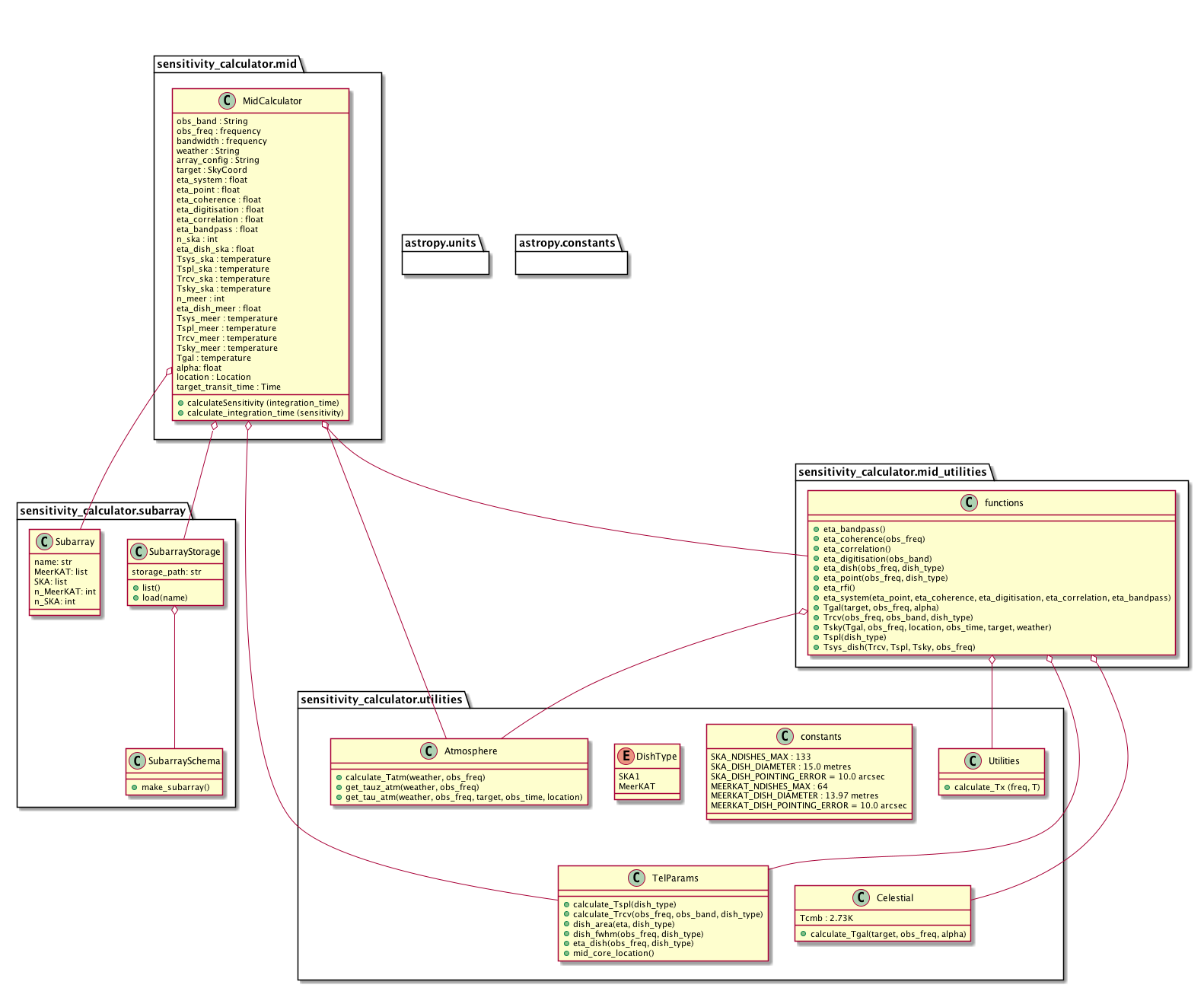
Figure 3 . Class diagram of the Sensitivity Calculator back-end.
The back-end is written in Python 3.7 and the class diagram is shown in Fig.3. The class MidCalculator has 2 public methods: calculate_sensitivity to get the array sensitivity in Jy for the given integration time, and calculate_integration_time to get the integration time required for the given sensitivity.
The MidCalculator constructor has a number of required parameters that define the observing configuration, target and weather. The rest default to None, in which case their values will be calculated automatically. The automatic values can be overriden by setting them here.
All parameters, internal variables and results that describe ‘physical’ measures are implemented as astropy Quantities to prevent mixups over units.
The calculator is modular in design. There are separate functions for deriving each element of the calculation, which can be easily modified as the sensitivity model is updated.
Front-end
Public and ‘Expert’ Users
The calculator is intended for two types of user.
The first type is the ordinary observer who will use the calculator to simply calculate the performance of the telescope when looking at their target object.
The second type is the ‘expert’ user, who understands the telescope design and wants to test the effect of tweaking some aspect of it. This mode of use is intended for SKA staff. It allows the user to manually edit some of the values which are usually calculated automatically as part of the sensitivity calculation. Say a user wanted to test out how a different array configuration might affect the sensitivity of a given observation. They could manually edit the number of SKA1 and MeerKAT dishes in the array and these would override the numbers that the calculator uses and use the new values in the sensitivity calculation. The diagram in Fig.4 shows the dependencies between the variables used in the sensitivity calculation. The variables coloured green are the ones which can be edited by the user in ‘expert’ mode; blue are calculated, and pink not yet implemented. The overall pattern matches that of the dependency tree in Fig.1, with some small differences which wil be eliminated in time.
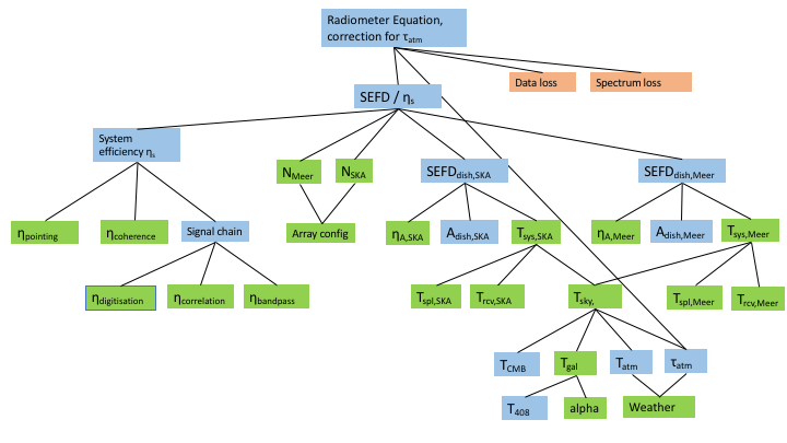
Figure 4 . Flowchart diagram showing the dependencies of the variables used in the sensitivity calculation.
Technologies
The calculator front-end is designed as a Flask web application, using Bootstrap 4 for a responsive design.
Flask is a WSGI web application framework, allowing for very simple interaction with the Python 3 back-end code. It also ensures that the sensitivity calculations are performed on the server-side, rather than the client-side. Currently the calculations are not computationally intense but as the calculator goes on to be developed and more features are added, there’s a good chance that this will change. In any case, having this setup minimises the amount of data to transfer between the user and the server, since, for example, when the program needs to access a lookup table hosted on the server, this file doesn’t need to be transferred to the user’s device. This will improve the speed of the calculator’s response and reduce the server load.
Bootstrap 4 is the most recent version of the Bootstrap toolkit - an open-source HTML, CSS and JS library allowing for quick and clean deployment of responsive web applications. Responsive design is extremely important to make sure that the webpage functions and looks good, regardless of the size/orientation of the user’s device. The calculator uses the Bootstrap 4 CDN (Content Delivery Network), which means that nothing needs to be installed on the server. When the user loads a page which uses the CDN, they may already have the required files cached on their device after visiting another website using the CDN. Since Bootstrap is the world’s most popular web framework, it is likely this will be the case. If, however, the user does not have the files cached, they will be retrieved from the closest server to the user that is part of the network. This means that there may be a little extra load-time when the user first visits the website, but overall load-time will be reduced from then on.
Typescript is the main client-side language. Along with some jQuery and AJAX to send RESTful requests to and from the server. Once the page is loaded there are two ‘entry points’ for the Typescript code to run. The first is when the “Calculate” button at the bottom of the page is clicked. Code will then run to read the information from the form, perform some validation (checking the inputs are formatted correctly, within some allowable ranges, etc.) before using AJAX to send the data using a GET request to the server-side Flask code. By performing this validation on the client side, we limit the number of unnecessary requests to the server, i.e. sending inputs which would not be allowed. The Flask code will parse the inputs and, based on the data sent, call the calculator back-end code to perform the necessary calculation, then return the results to the client-side, which will output them to the user’s screen. The other ‘entry point’ into the client-side code is when the user modifies one of the inputs. Once a value is changed and that input is deselected, some Typescript code will execute to perform similar validation. This helps make it clear what the actual values are that go into the calculator when the “Calculate” button is pressed.
There is also some custom CSS used to style the site. While bootstrap takes care of a lot of this, there are some tweaks which are made, such as setting the colours of the webpage to match those laid out in the SKA Brand Guidelines.
Inputs
The calculator inputs can be categorised by the observing mode they fall under. Universal inputs are those that apply regardless of the selected observing mode.
Universal
Observing Band The selected band to use for the observation:
Band 1: 0.35GHz - 1.05GHz
Band 2: 0.95GHz - 1.76GHz
Band 5a: 4.6GHz - 8.4GHz
Band 5b: 8.4GHz - 15.4GHz
Right Ascension and Declination The equatorial coordinates of the observed source. The sensitivity is calculated for the time at which the target reaches its maximum elevation, crossing the meridian.
Array Configuration Preset list of array configurations. Click on the tab to choose from:
full: all SKA1 and MeerKAT antennas
core: just the MeerKAT antennas
extended: just the SKA1 antennas
custom: activates the nSKA and nMeer fields where the user can enter the number of SKA and MeerKAT antennas directly.
Weather PWV If no value is set in the weather PWV (Precipitable Water Vapour) field then results will be given for 3 canonical conditions; “Good” (PWV=5mm), “Average” (PWV=10mm) and “Bad” (PWV=20mm). The PWV is used in the calculation of the atmospheric brightness temperature, \(T_{atm}\). Since \(T_{sys}\) is dependent on \(T_{sky}\) and therefore \(T_{atm}\) and the weather conditions, if the user decides to manually edit \(T_{sys}\) in ‘commisioning mode’, or any of the variables it depends on, the option to set the PWV will be removed.
Elevation The user can use this field to specify the elevation at which the target will be observed. If no value is set then a default of 45 degrees is assumed. If the given elevation is never reached by the target, then the target’s zenith elevation will be used. The actual elevation assumed for the sensitivity calculation is reported in the result table.
Integration Time Override This is an optional input, which can be left blank. If a value is entered, it will take precedence over any integration time inputs for any of the observing modes. This is useful if the user wants to test one integration time for multiple observing modes at once (so they don’t have to edit each one individually). It may be good to have the other integration time inputs disabled when a value is entered here.
‘Commissioning Mode’ Inputs As shown in Fig.5, the calculator in ‘commissioning’ mode allows the user to modify some of the variables used in the sensitivity calculation. The calculator front-end automatically enables/disables inputs to avoid conflicts as the user selects which one they want to edit. These are passed to the calculator back-end as hard-coded values which will be used in place of automatically calculating values for those variables.

Figure 5 . Expanded view of the additional inputs available in ‘commissioning’ mode.
Line
Zoom Frequency For each zoom, the user can input a frequency for that zoom. When a value is entered, the next zoom becomes enabled, allowing a value to be entered. It can however be left blank, and the calculation will only be done for zooms which have a set frequency. This way, the user can select how many zooms they want (up to a maximum, currently 4).
Zoom Resolution For each zoom, the user can set a line resolution.
Integration Time The integration time of the observation. Used when calculating the sensitivity that observing for this amount of time will achieve.
Sensitivity The sensitivity for the observation. Used when calculating the integration time necessary to achieve this sensitivity.
Supplied Toggle allowing the user to swap between integration time and sensitivity as the input (giving the other as the output).
Continuum
Central Frequency The central frequency for the observation. Must be within the selected band.
Bandwidth The bandwidth for the observation. Must be fully contained within the selected band.
Resolution The line resolution.
Number of chunks The user can select an integer number of chunks to split the bandwidth up into. If they do, the output report will show the sensitivity (or integration time) for each chunk.
Integration Time The integration time of the observation. Used when calculating the sensitivity that observing for this amount of time will achieve.
Sensitivity The sensitivity for the observation. Used when calculating the integration time necessary to achieve this sensitivity.
Supplied Toggle allowing the user to swap between integration time and sensitivity as the input (giving the other as the output).
Subarray lookup service
There is a subarray lookup service implemented as a REST API. The json files with the different subarray configuration are stored in a local folder in the server. The list of available subarray configurations can be retrieved from \subarrays. The idea is to populate the subarray dropdown menu using this service. In the future the service can be expanded to accept custom subarray configurations.